Bayesian Statistics 101 for Dummies like Me
If you are in some field that has data (which is a lot of fields these days), you will have undoubtedly encountered the term Bayesian statistics at some point. When I first encountered it, I did what most people probably do. I googled “What is Bayesian statistics?”. After reading through some resources and getting through the idiosyncratic terms/concepts (e.g. conjugate priors, posteriors, Markov Chain Monte Carlo), I still went away not really understanding what was so important about Bayesian statistics. This medium article is an attempt by me to know if my understanding is correct and also know if there is another application of Causal inference with Machine learning. Although I’ve tried my best to make it align with the 101 for Dummies like Me series, but this topic needed some coding experience for validation.
I’m all ‘bout that uncertainty, ‘bout that uncertainty, no certainty
That was my lame and sad attempt at trying to come up with some catching section name (inspired by Meghan Trainor’s “All About That Bass”) to describe the crux of Bayesian statistics.
But joking aside, the one concept that is fundamental to Bayesian statistics is that it’s all about representing uncertainty about an unknown quantity. To illustrate this, imagine I had a coin and I asked you what is the probability that the coin gives a Head if I flip it? You most likely guessed 0.5, which is a reasonable guess given your prior knowledge on how coins work. But what if I told you that I got this coin from a magic shop? You’ll probably have some doubts that it is 0.5 now. It could be anything now. Maybe it’s a trick coin that always gives you head (i.e. 1 probability)? Or maybe it always gives you a tail (i.e. 0 probability)? Or maybe it is biased towards some value (e.g. 0.75 probability). The point is there is some uncertainty in your estimation of this unknown quantity.
How do we represent these uncertainties?
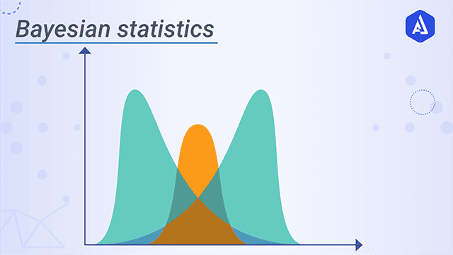
We have just learned that it’s all about the uncertainty in our estimations. So how do we actually represent these uncertainties? They are expressed as a probability distribution. For instance, imagine you had the following probability distribution:
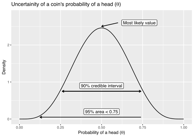
The x-axis represents the plausible values that θ could take. The y-axis represents the “confidence” (this isn’t entirely accurate in mathematical terms, but will suffice for this example) that the probability of a head takes this value. By expressing our uncertainty as a probability distribution, we get these benefits:
- The x value with the highest density peak represents the most likely value. In this case, that would be 0.5.
- Credible intervals (CI) can be formed. For instance, [0.25–0.75] forms a 90% CI that tells us we are 90% confident that the parameter is in this interval. This is quite different from a confidence interval in classical statistics, which is actually quite a counter-intuitive statistic.
- No p-value calculations. Just calculate the relevant tail areas. For instance, what is P(θ)<0.75? We just look at the area left of 0.75, which ends up being 0.95 of the total area. So we can say there is a 95% chance of P(θ)<0.75.
- There is a technique called Bayesian inference that allows us to adapt the distribution in light of additional evidence. This ultimately means we can update our estimation of our quantity when we get more data while still accounting for our prior information on the quantity.
Where do these probability distributions for representing uncertainty come from?
While you could theoretically make your own probability distributions, in practice people use established probability distributions (e.g. beta, normal). For instance, here are 6 different beta distributions:
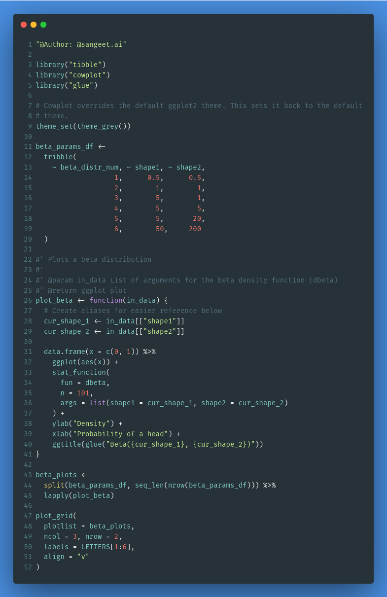
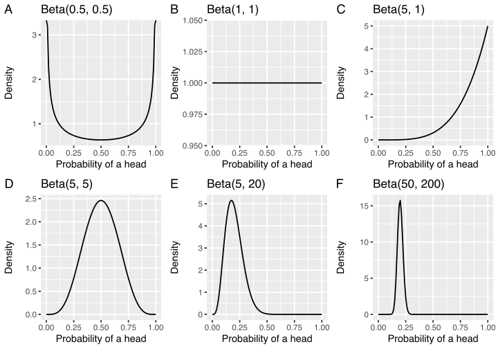
Each of these beta distributions represents different prior knowledge. For instance, Beta(0.5, 0.5) represents a belief that the coin always gives heads or tails. Beta(1, 1) represents a global uncertainty in that the probability of a head could be any value (this is often referred to as a uniform prior). Beta(50, 200) represents a strong belief that the probability is 0.2 for getting a Head.
Which type of distribution (e.g. beta, normal) depends on the type of data you are modeling.
So what do I do with this uncertainty probability distribution?
If we go back to the original scenario with the coin and recall this equation representing the number of expected heads:
rn∼Binomial(θ,n)rn∼Binomial(θ,n)
Rather than having our θ value as a single point estimate, we have it represented as a probability distribution representing all possible estimates with associated levels of uncertainty. This is effectively what Bayesian statisticians mean when they say setting a prior on an uncertain parameter. In this case, we will use a beta distribution as our prior.
It’s worth noting that in theory you can use any distribution. However in practice, certain prior distributions are used for specific models because it makes the math easier. These are called conjugate priors. I won’t go into the details in this post, but is worth knowing this if you come across this term.
So what we will literally do here is substitute the beta distribution into the binomial distribution (this forms what is called a beta-binomial) and then we can generate some expected outcomes. As you might guess, the shape of your beta will influence your expected outcomes. For instance, here we test the different effects of the 6 beta distributions on the distribution of the expected number of heads if we were to flip a coin 20 times across 1000 simulations (i.e. Monte Carlo simulation):
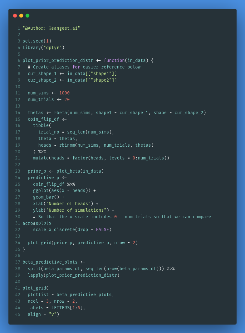
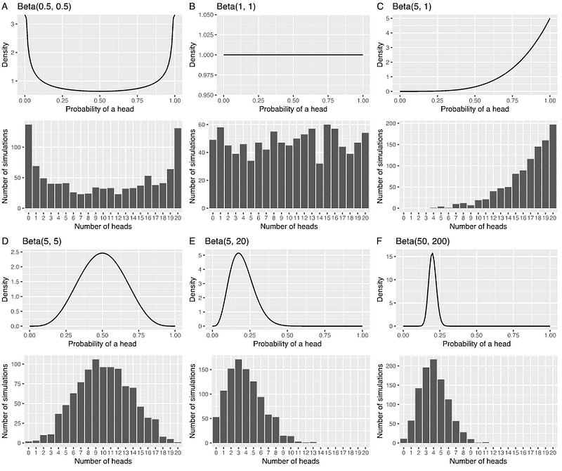
In each panel, the top plot is the beta prior distribution representing the uncertainty in your θ parameter for your binomial. Then the bottom plot is an approximate beta-binomial distribution of heads you would get if you use the corresponding beta prior (its an approximation because we are running a Monte Carlo simulation to estimate the distribution). This bottom plot is formally called a prior predictive distribution. As you can see, the bottom plots end up following the shape of the beta prior, which is actually what you would expect.
Conclusion
You’ve made it to the end of the post! Hopefully, this post helped illuminate the key concept of Bayesian statistics. Remember that it is all about representing uncertainty regarding an unknown quantity. This uncertainty is an expression as a probability distribution and ultimately impacts your expected outcome. As probability distributions are used, this is what makes Bayesian statistics fundamentally probabilistic.