Probability Theory 101 for Dummies like Me

In the Classical interpretation Probability is the measure of the likelihood that an event will occur in a Random Experiment; In other words, the frequency of the event occurring. Probability is quantified as a number between 0 and 1, where, loosely speaking, 0 indicates impossibility and 1 indicates certainty. The higher the probability of an event, the more likely it is that the event will occur. A simple example is the tossing of a fair (unbiased) coin. Since the coin is fair, the two outcomes (“heads” and “tails”) are both equally probable; the probability of “heads” equals the probability of “tails”; and since no other outcomes are possible, the probability of either “heads” or “tails” is 1/2 (which could also be written as 0.5 or 50%).
Probability is often associated with at least one event. This event can be anything. Toy examples of events include rolling a dieorpulling a colored ball out of a bag.In these examples the outcome of the event is random (you can’t be sure of the value that the die will show when you roll it), so the variable that represents the outcome of these events is called a random variable (often abbreviated to RV).
Key Probability concepts to get started
- Probability: the likelihood that an event will occur. For example, there is a 50% probability that a fair coin will come up heads on any given flip. Probabilities can be expressed as percents (30%), in decimal form (0.3) or in fractions (3/10). In statistics, we most often deal with probability as decimals.
- Probability(frequentist): over the long run, the proportion or percentage of time that an event will occur out of all observations. For example, I rolled one die a hundred times. Seventeen times out of a hundred the die showed a value of one. The probability of getting a one is therefore 0.17.
- Probability(subjective): a measure of the strength of belief. For example, the likelihood that it will storm this evening is 0.7, P(storm)=0.7.
- Random Variable: a variable (often denoted X) is a variable whose value is a function of a random process. In other words, the value is determined by chance or a stochastic process (can also think of as an experiment or data generating process). Here is a quick Khan Academy video on random variables.
- Discrete random variable: the random outcomes are countable(finite) and values between these counts can not occur. An example: A random variable, X, takes on the value of one if a coin shows heads, and zero if tails. The expected value or mean(μ) of a discrete random variable is ΣxP(x).
- Continuous random variable: outcomes and related probabilities are not defined at specific values, but rather over an interval of values. An example: A random variable, X, the weight of a fish caught from Kolkata, India, may range from 0.5 to 3.0 kg. The probability that an adult weighs between these values is the area under the curve of the probability density function.
- Sample space(S): the collection of all possible outcomes. The sample space for the rolling of a die is: S={1, 2, 3, 4, 5, 6}
- Complement: the probability of the complement of A includes the sum of all probabilities in the sample space that is not A. For example, the probability of the complement of rolling a five on a die(S={1,2,3,4,6}) equals 5/6.
- Mutually exclusive events: Two (or more) events that can not occur at the same time. P(A and B) = 0. Example: The Chicago Bulls basketball team can not both win(event A) and lose(event B) a game, therefore P(win and lose) or P(A and B) = 0. We also call these events disjoint.
- Independent events: If an event occurring does not alter the probability of another event occurring, we say that these events are independent. For example, if we roll a die twice, getting a three on the first roll does not affect the probability of getting a three on the second roll. Therefore, we can say that these two events are independent.
- Dependent events: if an event occurring(A) changes the probability of another event occurring(B), we can say that the probability of event B is dependent on event A. For example, the probability of elevated ground-level ozone concentrations is dependent on the occurrence of a large traffic jam. To learn more about independent and dependent events, please see Khan Academy’s website on dependent probabilities.
The Rules or Axioms in Probability Theory
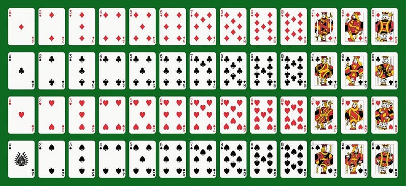
Before we get started on this section, let me introduce to you a deck of cards (inherited from the French several centuries ago). A deck is composed of 52 cards, half Red and half Black. The Red suits are Hearts and Diamonds while the Blacks are Spades and Clubs. There are 13 cards in each suit (Ace, 2, 3, 4, 5, 6, 7, 8, 9, 10, Jack, Queen and King). Ace may be either the highest or lowest card (depending on the game).
- A probability may range from zero (0) to one (1), inclusive.
- The probabilities of all possible outcomes must sum to one. This axiom can be written as:

This is the shorthand for writing ‘the sum (the sigma sign) of the probabilities(P) of all events (Ai) from i=0 to i=n equals one’.
- The probability of an event plus the probability of its complement must equal one.
The Addition Rule
So back to our deck of cards. We want to know the probability that a drawn card is either a red card(P(A)) OR a seven(P(B)). These two events are NOT mutually exclusive (i.e., a card can be Red AND a seven). So in this case,
P(A or B) = P(A) + P(B) — P(A and B)
P(red or seven) = p(red) + p(seven) — p(red and seven)
P(red or seven) = 26/52 + 4/52–2/52 = 28/52 = 7/13
We subtract the 7 of Hearts(Red) card and the 7 of Diamonds card(Red) because we don’t want to count these cards twice.
The Multiplication Rule
If two events are INDEPENDENT (the occurrence of one event does not affect the probability of another event occurring), then
P(A and B) = P(A)P(B)
An example of two INDEPENDENT events is two rolls of a die. The probability of getting a One on the first roll will not affect the probability of getting a One on the second roll. So if we roll the die twice and want to know the probability of getting a one on both rolls:
P(one (roll1) and one (roll2)) = P(one(roll1))*P(one(roll2)) = 1/6 * 1/6 = 1/36
The Law of Large Numbers
The law of large numbers (sometimes named the Law of Averages) states that as the number of trials of a random experiment increases, the empirical probability of an outcome will get closer and closer to its true probability. Or another way of thinking about it, as the number of random trials increases, the expected value of the trial outcomes will approach the true Population Mean.
So what does this mean? Let’s say we have a fair die, with sides numbered one through six, inclusive. We roll the die six times and count how many times a one appears. The true probability (if the die is fair) of getting a one on each individual trial is 1/6. However, with our 6 trials, three rolls produced a one (3/6). This is more often than is expected but not totally out of the realm of possibility (we could calculate the probability of this using our probability rules). We know the ‘true’ probability of getting a one on any roll is 1/6. What if we rolled the die 60 times? What’s the likelihood of getting 30 ones?!? Very, very small. We would expect the proportion of rolls coming up one to be closer to 1/6. And with 600 rolls, even closer to 1/6. As the number of trials increases, the long-term frequency, based on our empirical results, will approach the true probability. This is the law of large numbers.
The 3 types of Probability
In the earlier sections above I introduced the concept of a random variable and some notation on probability. However, probability can get quite complicated. Perhaps the first thing to understand is that there are different types of probability. It can either be marginal, joint or conditional.
Marginal Probability: If A is an event, then the marginal probability is the probability of that event occurring, P(A). Example: Assuming that we have a pack of traditional playing cards, an example of a marginal probability would be the probability that a card is drawn from a pack is red: P(red) = 0.5.
Joint Probability: The probability of the intersection of two or more events. Visually it is the intersection of the circles of two events on a Venn Diagram (see figure below). If A and B are two events then the joint probability of the two events is written as P(A ∩ B). Example: the probability that a card drawn from a pack is red and has the value 4 is P(red and 4) = 2/52 = 1/26. (There are 52 cards in a pack of traditional playing cards and the 2 red ones are the hearts and diamonds). We’ll go through this example in more detail later.
Conditional Probability: The conditional probability is the probability that some event(s) occur given that we know other events have already occurred. If A and B are two events then the conditional probability of A occurring given that B has occurred is written as P(A|B). Example: the probability that a card is a four given that we have drawn a red card is P(4|red) = 2/26 = 1/13. (There are 52 cards in the pack, 26 are red and 26 are black. Now because we’ve already picked a red card, we know that there are only 26 cards to choose from, hence why the first denominator is 26).
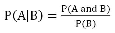
How to Manipulate among Joint, Conditional and Marginal
The equation below is a means to manipulate among joint, conditional and marginal probabilities. As you can see in the equation, the conditional probability of A given B is equal to the joint probability of A and B divided by the marginal of B. Let’s use our card example to illustrate. We know that the conditional probability of a four, given a red card equals 2/26 or 1/13. This should be equivalent to the joint probability of a red and four (2/52 or 1/26) divided by the marginal P(red) = 1/2. And low and behold, it works! As 1/13 = 1/26 divided by 1/2. For the diagnostic exam, you should be able to manipulate among joint, marginal and conditional probabilities.
Bayes’ Theorem
Bayes’ theorem: an equation that allows us to manipulate conditional probabilities. For two events, A and B, Bayes’ theorem lets us go from P(B|A) to P(A|B) if we know the marginal probabilities of the outcomes of A and the probability of B, given the outcomes of A. Here is the equation for Bayes’ theorem for two events with two possible outcome (A and not A).

Let’s assume we know that 1% of women over the age of 40 have breast cancer, P(cancer)=0.01, Let’s assume that 90% of women who have breast cancer will test positive for breast cancer in a mammogram, P(positive test|cancer)=0.9 Eight percent of women that do NOT have cancer will also test positive, P(positive test|no cancer)=0.08
What is the probability that a woman has cancer if she tests positive P(cancer|positive test)?
We will call P(cancer) = P(A), and the P(positive test) = P(B). We want to know P(A|B),the probability of having cancer if you have a positive test.
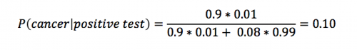
Using Bayes’ theorem, we calculate that the likelihood that a woman has breast cancer, given a positive test equals approximately 0.10. This makes intuitive sense as this result is greater than 1% (the percent of breast cancer in the general public).
Probability versus Statistics
Probability and statistics are related areas of mathematics which concern themselves with analyzing the relative frequency of events. Still, there are fundamental differences in the way they see the world:
- Probability deals with predicting the likelihood of future events, while statistics involves the analysis of the frequency of past events.
- Probability is primarily a theoretical branch of mathematics, which studies the consequences of mathematical definitions. Statistics is primarily an applied branch of mathematics, which tries to make sense of observations in the real world.

Both subjects are important, relevant, and useful. But they are different, and understanding the distinction is crucial in properly interpreting the relevance of mathematical evidence. Many a gambler has gone to a cold and lonely grave for failing to make the proper distinction between probability and statistics.
This distinction will perhaps become clearer if we trace the thought process of a mathematician encountering his first craps game:
If this mathematician were a probabilist, he would see the dice and think, “Six-sided dice? Presumably, each face of the dice is equally likely to land face up. Now assuming that each face comes up with probability 1/6, I can figure out what my chances of crapping out are.”
If instead, a statistician wandered by, he would see the dice and think, “Those dice may look OK, but how do I know that they are not loaded? I’ll watch a while, and keep track of how often each number comes up. Then I can decide if my observations are consistent with the assumption of equal-probability faces. Once I’m confident enough that the dice are fair, I’ll call a probabilist to tell me how to play.’’
In summary, probability theory enables us to find the consequences of a given ideal world, while statistical theory enables us to measure the extent to which our world is ideal.
Frequentist vs. Bayesian View
One thing that is worth mentioning is that in the introduction of this post I made a statement regarding the classic interpretation of probability. Specifically, this classic interpretation is referred to as the frequentist view of probability. In this view, probabilities are based purely on objective, random experiments with the assumption that given enough trials (long-run) the relative frequency of event x will equal to the true probability of x. Notice how all of the probabilities we reported in this post were based purely on the frequency.
If you’ve done any statistics or analytics, you’ll likely have come across the term Bayesian statistics. In brief, Bayesian statistics differ from the frequentists view in that it incorporates subjective probability which is the degree of belief in an event. This degree of belief is called the prior probability distribution and is incorporated along with the data from random experiments when determining probabilities.
Conclusion
Still wondering why you need to learn Probability Theory? In gambling, people often talk about how they initially won but ended up losing money in the end. Why does this happen? Probability has an answer to that.
Consider the game of Roulette. It has numbers 1–36 divided into two colors(Red & Black) and two additional numbers ‘0’ and ‘00’. You can bet on any specific given number, color, rows, or a few combinations of numbers. Here is how the numbers on the table are organized.
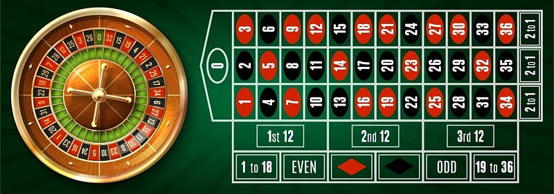
Winning criteria:
Let’s say I bet $10 on Even and the number 20 is picked then I basically doubled my investment. Returns are calculated based on the 36 colored numbers (1–36). If D is your investment, then returns are D * (36/X) where X is a count of numbers fitting the criteria. If I bet $10 on Even then there are 18 numbers fitting the criteria. So if I win I get back 10*(36/18) = 20. Similarly if I $10 bet on ‘2nd 12’ and win I get back 10 * (36/12) = 30 ($20 profit). If i bet $10 on 20 and win, then I get back 10*(36/1) = $360.
Looks like an evenly placed game right? No. It is structured to look like the chance of winning a number is 1 in 36 but in reality, it is 1 in 38 (due to ‘0’ and ‘00’). In other words, it takes a minimum of 38 chances to pick every number on the table.
Assume the following situation: We are betting $10 on the number 20 every time roulette is rolled. We are playing until all the numbers are picked and luckily it took us only 38 chances for all of them to be picked. Investment = 38 * $10 = $380. Winnings: we lost 37 times and won 1 time so our winning is 10 *(36/1) = $360. So for one full round of the game, we lost $20. If the number of times we play the game is significantly large then we can only lose money on the table and not win. How did I get to this conclusion? Probability.
In the above scenario, the best strategy to win money would be to stop playing if you won money early in the game. Let’s say number 20 was picked on the 25th roll. Then total investment is $250 and returns are $360 where I am still winning $110. This is only one of the many everyday practical applications of Probability.
- Why do Turtles lay a large number of eggs? Probability of Hatching and Survival determine this for its species to continue.
- Among humans, is there a correlation between Life Expectancy and the Average number of children per family. I bet there would be, there are several other factors such as income, economy etc that would affect this.
- What is the chance of me passing a multiple-choice test if I go unprepared to test?