Dimensionality Reduction 101 for Dummies like Me
Let’s starts with the WHY we need to perform Dimensionality Reduction before analyzing data and coming down to some inferences, it is often necessary to visualize the data set, in order to get an idea of it. But, nowadays data sets contain a lot of random variables (also called features) due to which it becomes difficult in visualizing the data set. Sometimes it is even impossible to visualize such high dimensional data as we humans fall astray after we reach a dimension higher than 3. Here is where we come across dimensionality reduction. As the name suggests it is:
The process of reducing the number of random variables of the data set under consideration, via obtaining a set of principal variables.
Why is Dimensionality Reduction so important?
Consider this scenario where you have a need for a lot of indicators variables in your dataset to reach a more accurate result from your machine learning model, then you tend to add as many features as possible at first. However, after a certain point, the performance of the model will decrease with the increasing number of elements. This phenomenon is often referred to as “The Curse of Dimensionality.”
The curse of dimensionality occurs because the sample density decreases exponentially with the increase of the dimensionality. When we keep adding features without increasing the number of training samples as well, the dimensionality of the feature space grows and becomes sparser and sparser. Due to this sparsity, it becomes much easier to find a “perfect” solution for the machine learning model which highly likely leads to overfitting.
Overfitting happens when the model corresponds too closely to a particular set of data and doesn’t generalize well. An overfitted model would work too well on the training dataset so that it fails on future data and makes the prediction unreliable. So how could we overcome the curse of dimensionality and avoid overfitting especially when we have many features and comparatively few training samples? This is where dimensionality reduction techniques come to rescue. Broadly, dimensionality reduction has two classes — feature elimination and feature extraction.
Feature elimination which is the removal of some variables completely if they are redundant with some other variable or if they are not providing any new information about the data set. The advantage of feature elimination is that it is simple to implement and makes our data set small, including only variables in which we are interested. But as a disadvantage — we might lose some information from the variables which we dropped.
Feature extraction, on the other hand, is the formation of new variables from the old variables. Say, you have 29 variables in your data set, then feature extraction technique will create 29 new variables which are combinations of 29 old variables. PCA is the example of one such feature extraction method. Below is an image classifying the different Dimensionality Reduction techniques:
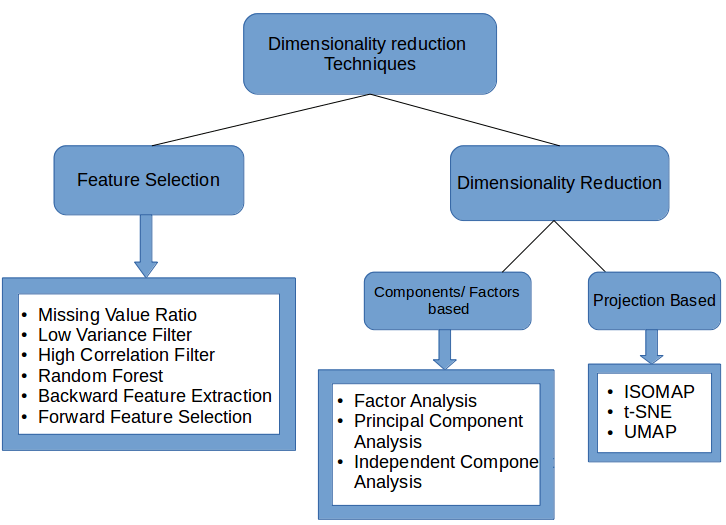
Image Source: https://www.analyticsvidhya.com/blog/2018/08/dimensionality-reduction-techniques-python/
- Missing Values Ratio: Data columns with too many missing values are unlikely to carry much useful information. Thus, data columns with a ratio of missing values greater than a given threshold can be removed. The higher the threshold, the more aggressive the reduction.
- Low Variance Filter: Similar to the previous technique, data columns with little changes in the data carry little information. Thus, all data columns with a variance lower than a given threshold can be removed. Notice that the variance depends on the column range, and therefore normalization is required before applying this technique.
- High Correlation Filter: Data columns with very similar trends are also likely to carry very similar information, and only one of them will suffice for classification. Here we calculate the Pearson product-moment correlation coefficient between numeric columns and the Pearson’s chi-square value between nominal columns. For the final classification, we only retain one column of each pair of columns whose pairwise correlation exceeds a given threshold. Notice that correlation depends on the column range, and therefore, normalization is required before applying this technique.
- Random Forests/Ensemble Trees: Decision tree ensembles, often called random forests, are useful for column selection in addition to being effective classifiers. Here we generate a large and carefully constructed set of trees to predict the target classes and then use each column’s usage statistics to find the most informative subset of columns. We generate a large set (2,000) of very shallow trees (two levels), and each tree is trained on a small fraction (three columns) of the total number of columns. If a column is often selected as the best split, it is very likely to be an informative column that we should keep. For all columns, we calculate a score as the number of times that the column was selected for the split, divided by the number of times in which it was a candidate. The most predictive columns are those with the highest scores.
- Backward Feature Elimination: In this technique, at a given iteration, the selected classification algorithm is trained on ninput columns. Then we remove one input column at a time and train the same model on n-1columns.*The input column whose removal has produced the smallest increase in the error rate is removed, leaving us with *n-1 input columns. The classification is then repeated using n-2 columns, and so on. Each iteration k produces a model trained on n-k columns and an error rate e(k).By selecting the maximum tolerable error rate, we define the smallest number of columns necessary to reach that classification performance with the selected machine learning algorithm.
- Forward Feature Construction: This is the inverse process to backward feature elimination. We start with one column only, progressively adding one column at a time, i.e., the column that produces the highest increase in performance. Both algorithms, backward feature elimination, and forward feature construction are quite expensive in terms of time and computation. They are practical only when applied to a dataset with an already relatively low number of input columns.
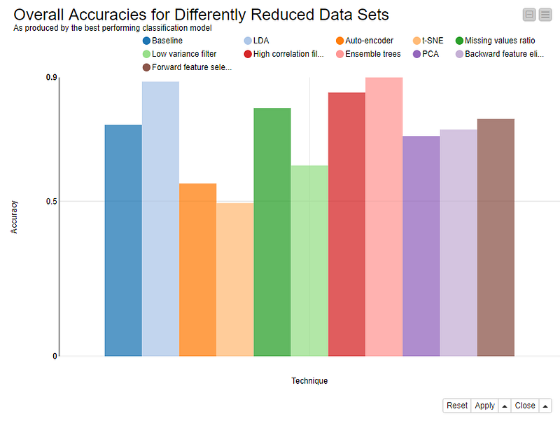
Figure 1. Accuracies of the best-performing models trained on well-known datasets that were reduced using the 10 selected data dimensionality reduction techniques.
Linear Dimensionality Reduction Methods
The most common and well-known dimensionality reduction methods are the ones that apply linear transformations, like
- Factor Analysis: This technique is used to reduce a large number of variables into fewer numbers of factors. The values of observed data are expressed as functions of a number of possible causes in order to find which are the most important. The observations are assumed to be caused by a linear transformation of lower-dimensional latent factors and added Gaussian noise.
- Principal Component Analysis (PCA): Principal component analysis (PCA) is a statistical procedure that orthogonally transforms the original nnumeric dimensions of a dataset into a new set of ndimensions called principal components. As a result of the transformation, the first principal component has the largest possible variance; each succeeding principal component has the highest possible variance under the constraint that it is orthogonal to (i.e., uncorrelated with) the preceding principal components. Keeping only the first m < nprincipal components reduces the data dimensionality while retaining most of the data information, i.e., variation in the data. Notice that the PCA transformation is sensitive to the relative scaling of the original columns, and therefore, the data need to be normalized before applying PCA. Also notice that the new coordinates (PCs) are not real, system-produced variables anymore. Applying PCA to your dataset loses its interpretability. If interpretability of the results is important for your analysis, PCA is not the transformation that you should apply.
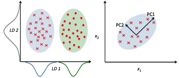
Figure 2.PCA orients data along the direction of the component with maximum variance whereas LDA projects the data to signify the class separability
- LDA (Linear Discriminant Analysis): projects data in a way that the class separability is maximized. Examples from the same class are put closely together by the projection. Examples from different classes are placed far apart by the projection.
Non-linear Dimensionality Reduction Methods
Non-linear transformation methods or manifold learning methods are used when the data doesn’t lie on a linear subspace. It is based on the manifold hypothesis which says that in a high dimensional structure, the most relevant information is concentrated in a small number of low dimensional manifolds. If a linear subspace is a flat sheet of paper, then a rolled-up sheet of paper is a simple example of a nonlinear manifold. Informally, this is called a Swiss roll, a canonical problem in the field of non-linear dimensionality reduction. Some popular manifold learning methods are,
- Multi-dimensional scaling (MDS): A technique used for analyzing similarity or dissimilarity of data as distances in a geometric space. Projects data to a lower dimension such that data points that are close to each other (in terms of Euclidean distance) in the higher dimension are close in the lower dimension as well.
- Isometric Feature Mapping (Isomap): Projects data to a lower dimension while preserving the geodesic distance (rather than Euclidean distance as in MDS). Geodesic distance is the shortest distance between two points on a curve.
- Locally Linear Embedding (LLE): Recovers global non-linear structure from linear fits. Each local patch of the manifold can be written as a linear, weighted sum of its neighbors given enough data.
- Hessian Eigenmapping (HLLE): Projects data to a lower dimension while preserving the local neighborhood like LLE but uses the Hessian operator to better achieve this result and hence the name.
- Spectral Embedding (Laplacian Eigenmaps): Uses spectral techniques to perform dimensionality reduction by mapping nearby inputs to nearby outputs. It preserves locality rather than local linearity
- t-distributed Stochastic Neighbor Embedding (t-SNE): Computes the probability that pairs of data points in the high-dimensional space are related and then chooses a low-dimensional embedding which produces a similar distribution.
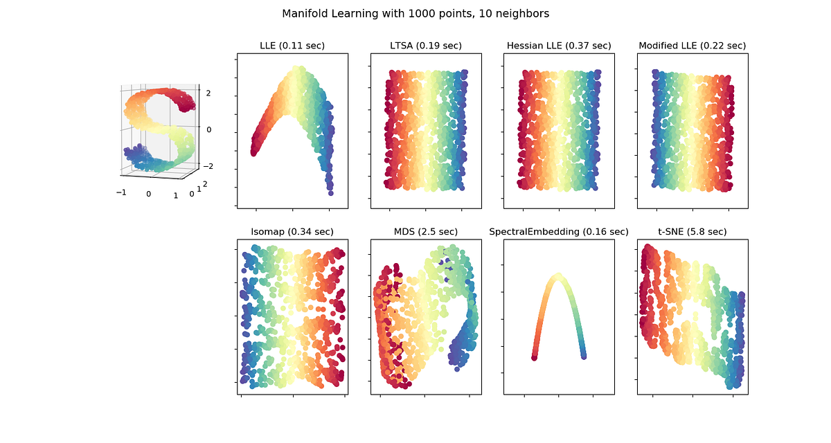
Figure 3.Shows the resulting projection from applying different manifold learning methods on a 3D S-Curve. Image Source: https://scikit-learn.org/stable/modules/manifold.html
Is Dimensionality Reduction GOOD or BAD?
There is no global right or wrong answer. It depends on the situation to situation. Let me cover a few examples to bring out the spectrum of possibilities. These may not be comprehensive but would give you a good flavor of what should be done.
Example 1: We are building a regression with 10 variables, some of
them are mildly correlated.
In this case, there is no need to perform any dimensionality reduction.
Since there is little correlation between the variables, all of them are
bringing in new information. We should keep all the variables in the mix
and build a model.
Example 2: Again, we are building a regression model. This time with
20 variables and some of these variables are highly correlated.
For example, in the case of telecom — the number of calls made by a
customer in a month and the monthly bill he/she receives. Or in case of
insurance, it could be the number of policies and total premium sold by
an agent/branch. In these cases, because you only have a limited number
of variables you should only add one of these variables to your model.
There is limited / no value you might get by bringing in all the
variables. And a lot of this additional value can be noise. You can
still do away with applying any formal dimensional reduction technique
in this case (even though you are doing it for all practical reasons).
Example 3: Now assume that we have 500 such variables with some of
them being correlated with each other.
For example, the data output of sensors from a smartphone. Or a retail
chain looking at the performance of a store manager with tons of similar
variables — like the total number of SKUs sold, number of bills created,
number of customers sold to, number of days present, time spent on the
aisle, etc. etc. All of these would be correlated and are way too many
to individually figure out which are correlated to which ones. In this
case, you should definitely apply dimension reduction techniques. You
may or may not make actual sense of these vectors, but you can still
understand them by looking at the result.
In a lot of scenarios like this, you will also see that you will retain
more than 90% of information with less than 15–20% of variables. Hence,
these can be good applications of dimensionality reduction.
Auto Encoders for Dimensionality Reduction
While PCA and t-SNE are methods, Auto Encoders are a family of methods.
Auto Encoders are neural networks where the network aims to predict the
input (the output is trained to be as similar as possible to the input)
by using less hidden nodes (on the end of the encoder) than input nodes
by encoding as much information as it can to the hidden nodes.
A basic Auto Encoder for our 4-dimensional iris dataset would look like
Figure 4 below, where the lines connecting between the input layer to
the hidden layer are called the “encoder” and the lines between the
hidden layer and the output layer the “decoder”.
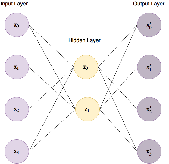
Figure 4. Basic Auto Encoder for the iris dataset
So why are Auto Encoders are a family? Well because the only constraint we have is that the input and output layer will be of the same dimension, inside we can create any architecture we want to be able to encode best our high dimensional data.
Auto Encoders starts with some random low dimensional representation (z) and will gradient descent towards their solution by changing the weights that connect the input layer to the hidden layer, and the hidden layer to the output layer.
By now we can already learn something important about Auto Encoders
because we control the inside of the network, we can engineer encoders
that will be able to pick very complex relationships between features.
Another great plus in Auto Encoders, is that since by the end of the
training we have the weights that lead to the hidden layer, we can train
on certain input, and if later on, we come across another data point we
can reduce its dimensionality using those weights without
re-training — but be careful with that, this will only work if the data
point is somewhat similar to the data we trained on.
To explore the math of Auto Encoder could be simple in this case but not
quite useful since the math will be different for every architecture and
cost function we will choose. But if we take a moment and think about
the way the weights of the Auto Encoder will be optimized we understand
the cost function we define has a very important role.
Since the Auto Encoder will use the cost function to determine how good
are its predictions we can use that power to emphasize what we want to.
Whether we want the euclidean distance or other measurements, we can
reflect them on the encoded data through the cost function, using
different distance methods, using asymmetric functions and whatnot.
More power lies in the fact that as this is a neural network
essentially, we can even weight classes and samples as we train to give
more significance to certain phenomenons in the data. his gives us great
flexibility in the way we compress our data.
Auto Encoders are very powerful and have shown some great results in comparison to other methods in some cases (just Google “PCA vs Auto Encoders”) so they are definitely a valid approach.
Visualizing High Dimensional Data
Self-Organizing Maps (SOM)
It is a type of artificial neural network (ANN) that is trained using unsupervised learning to produce a low-dimensional (typically two-dimensional), discretized representation of the input space of the training samples, called a map, and is, therefore, a method to do dimensionality reduction. Self-organizing maps differ from other artificial neural networks as they apply competitive learning as opposed to error-correction learning (such as backpropagation with gradient descent), and in the sense that they use a neighborhood function to preserve the topological properties of the input space. SOMwas introduced by Finnish professor Teuvo Kohonen in the 1980s is sometimes called a Kohonen map.
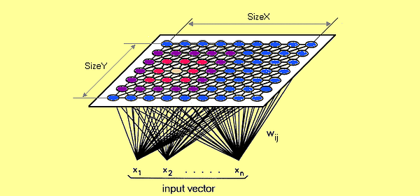
Image Source: https://www.google.com
Each data point in the data set recognizes themselves by competing for representation. SOM mapping steps starts from initializing the weight vectors. From there a sample vector is selected randomly and the map of weight vectors is searched to find which weight best represents that sample. Each weight vector has neighboring weights that are close to it. The weight that is chosen is rewarded by being able to become more like that randomly selected sample vector. The neighbors of that weight are also rewarded by being able to become more like the chosen sample vector. This allows the map to grow and form different shapes. Most generally, they form square/rectangular/hexagonal/L shapes in 2D feature space.
Sammon’s Mapping
Sammon’s mapping is one of the most popular metric, nonlinear dimensionality reductions method widely applied in visualizing high dimensional data. It is a simple yet very useful nonlinear projection algorithm that maps the high dimensional (𝑛) features in the original data into fewer variables (𝑚 dimensions,𝑚 < 𝑛) by preserving the inherent structure of the data. Generally speaking, Sammon mapping attempts to preserve the structure of high(𝑛) dimensional data by finding 𝑁 points in a much lower (𝑚) dimensional data space such that the inter-point distance measured in the 𝑚-dimensional space, approximate the corresponding inter-point distance in the 𝑛-dimension space. While PCA tries to preserve the variance of the data, Sammon mapping tries to preserve the inter-pattern distances by optimizing a cost function that describes how well the pairwise distances in a dataset are preserved. This can be achieved by minimizing an error criterion, called Sammon’s stress.
T-Distributed Stochastic Neighbouring Entities (t-SNE)
t-Distributed Stochastic Neighbor Embedding (t-SNE) is another technique for dimensionality reduction and is particularly well suited for the visualization of high-dimensional datasets. Contrary to PCA it is not a mathematical technique but a probabilistic one. The original paper describes the working of t-SNE as:
“t-Distributed stochastic neighbor embedding (t-SNE) minimizes the divergence between two distributions: a distribution that measures pairwise similarities of the input objects and a distribution that measures pairwise similarities of the corresponding low-dimensional points in the embedding”.
Essentially what this means is that it looks at the original data that is entered into the algorithm and looks at how to best represent this data using fewer dimensions by matching both distributions. The way it does this is computationally quite heavy and therefore there are some (serious) limitations to the use of this technique. The other key drawback is that it:
“Since t-SNE scales quadratically in the number of objects N, its applicability is limited to data sets with only a few thousand input objects; beyond that, learning becomes too slow to be practical (and the memory requirements become too large)”.