PyTorch 101 for Dummies like Me

What is PyTorch?
It’s a Python-based package to serve as a replacement for Numpy arrays and to provide a flexible library forDeep Learning Development Platform. As for the why I prefer PyTorch over TensorFLow can be learned from this Fast AI’s blog post for the reason to switch to PyTorch. Or simply put, the major reason according to me is having Dynamic computation graphs, which makes debugging neural networks easier for users.
What is a Matrix?
A matrix is a grid of n × m (say, 4× 4), where we can add and subtract matrices of the same size, multiply one matrix with another as long as the sizes are compatible ((n × m) × (m× p) = n × p), and multiply an entire matrix by a constant. A vector is a matrix with just one row or column, so there are a bunch of mathematical operations that we can do to any matrix.
What is a Numpy array in Python?
Numpy is the core library for scientific computation in Python. It provides a high-performance multidimensional array object and tools for working with these arrays. A numpy array is a grid of values, all of the same type, and is indexed by a tuple of nonnegative integers. The number of dimensions is the rank of the array; the shape of an array is a tuple of integers giving the size of the array along each dimension. To know more about how Numpy works please refer to this link.
Why Tensors and not Numpy?
The reason why we use Numpy in Machine Learning is that it’s much faster than Python lists at doing matrix ops. Why? Because it does most of the heavy lifting in C. But, in case of training deep neural nets, NumPy arrays alone would take months to train some of the state-of-the-art networks. This is where Tensors come into play. PyTorch provides us with a data structure called a Tensor, which is very similar to NumPy’s ND-array.But unlike the latter, tensors can tap into the resources of a GPU to significantly speed up matrix operations.
Tensors are multi-dimensional Matrices.
``` {#77dd .graf .graf–pre .graf-after–p name=”77dd”} torch.Tensor(x, y)
This will create an X by Y dimensional Tensor that has been instantiated
with random values. To Create a 7x5 Tensor with values randomly selected
from a Uniform Distribution between -1 and 1,

``` {#c3c3 .graf .graf--pre .graf-after--p name="c3c3"}
torch.Tensor(7, 5).uniform_(-1, 1)
Tensors have a size attribute that can be called to check their size
``` {#804c .graf .graf–pre .graf-after–p name=”804c”} print(x.size())
PyTorch supports various Tensor Functions with different syntaxes:

Consider Addition:

-   Normal Addition

``` {#e834 .graf .graf--pre .graf-after--li name="e834"}
y = torch.rand(5, 3)print(x + y)
- Getting Result in a Tensor
``` {#3274 .graf .graf–pre .graf-after–li name=”3274”} result = torch.Tensor(5, 3)torch.add(x, y, out=result)
-   In Line

``` {#0270 .graf .graf--pre .graf-after--li name="0270"}
y.add_(x)
Inline functions are denoted by an underscore following their name. Note: These have faster execution time (With a higher memory complexity tradeoff)
All Numpy Indexing, Broadcasting and Reshaping functions are supported
Note: PyTorch doesn’t support a negative hop so [::-1] will result in an error
``` {#16e1 .graf .graf–pre .graf-after–p name=”16e1”} print(x[:, 1])
``` {#4000 .graf .graf--pre .graf-after--pre name="4000"}
y = torch.randn(5, 10, 15)print(y.size())print(y.view(-1, 15).size())
For more detail on the difference between a numpy array and a Tensor go through this well-written post on Medium.
What are computational graphs?
A computational graph is a directed graph where the nodes correspond to operations or variables. Variables can feed their value into operations, and operations can feed their output into other operations. This way, every node in the graph defines a function of the variables. The computation graph is simply a data structure that allows you to efficiently apply the chain rule to compute gradients for all of your parameters. Suppose, your model is described like this:
``` {#48d5 .graf .graf–pre .graf-after–p name=”48d5”} b = w1 * ac = w2 * a d = (w3 * b) + (w4 * c)L = f(d)
If I were to actually draw the computation graph, it would probably look
like this.

**NOW**, you must note, that the above figure is not entirely an
accurate representation of how the graph is represented under the hood
by PyTorch. However, for now, it’s enough to drive our point home.
Why should we create such a graph when we can sequentially execute the
operations required to compute the output?
Imagine, what was to happen, if you didn’t merely have to calculate the
output but also train the network. You’ll have to compute the gradients
for all the weights labeled by purple nodes. That would require you to
figure your way around chain rule, and then update the weights.
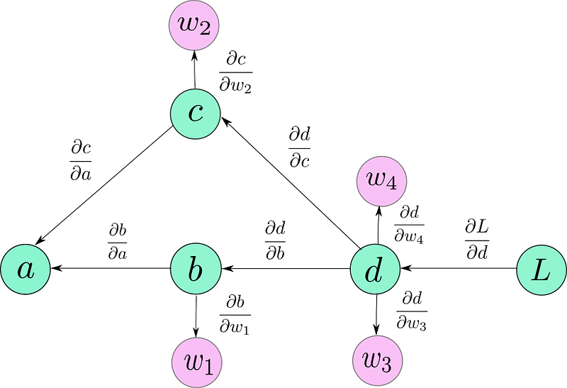
Here are a couple of things to notice. First, that the directions of the
arrows are now reversed in the graph. That’s because we are
backpropagating, and arrows mark the flow of gradients backward.
Second, for the sake of these examples, you can think of the gradients I
have written as *edge weights*. Notice, these gradients don’t require
chain rule to be computed.
Now, in order to compute the *gradient of any node, say, L, with respect
of any other node, say c ( dL / dc)*all we have to do is.
1. Trace the path *from L to c*. This would be*L → d → c.*
2. Multiply all the *edge weights* as you traverse along this path. The
quantity you end up with is: ( *dL / dd ) \**( *dd / dc ) = ( dL /
dc)*
3. If there are multiple paths, add their results. For example, in the
case of *dL/da,*we have two paths.*L → d → c → a and L → d → b→
a.*We add their contributions to get the gradient of*L w.r.t. a.*
*[*( *dL / dd ) \**( *dd / dc ) \**( *dc / da )]*+ *[*( *dL / dd ) \**(
*dd / db ) \**( *db / da )]*
In principle, one could start at *L*, and start traversing the graph
backward, calculating gradients for every node that comes along the way.
This
[video](https://www.coursera.org/lecture/neural-networks-deep-learning/computation-graph-4WdOY)
by Dr. Andrew Ng. gives a very good overview of computation graphs.
### What are Variables and autograd?
#### Autograd: automatic differentiation
The `autograd`{.markup--code .markup--p-code} package provides automatic
differentiation for all operations on Tensors. It is a define-by-run
framework, which means that your backprop is defined by how your code is
run and that every single iteration can be different.
#### Variable
`autograd.Variable`{.markup--code .markup--p-code} is the central class
of the package. It wraps a Tensor and supports nearly all of the
operations defined on it. Once you finish your computation you can
call `.backward()`{.markup--code .markup--p-code} and have all the
gradients computed automatically.
You can access the raw tensor through the `.data`{.markup--code
.markup--p-code} attribute, while the gradient w.r.t. this variable is
accumulated into `.grad`{.markup--code .markup--p-code}.
``` {#984f .graf .graf--pre .graf-after--p name="984f"}
x_data = [1.0, 2.0, 3.0]y_data = [2.0, 4.0, 6.0]w = Variable(torch.Tensor([1.0]), requires_grad=True)
Calling the Backward function
{#df5b .graf .graf--pre .graf-after--p name="df5b"}
l = loss(x_val, y_val)l.backward()
You can’t access the gradattribute of non-leaf Variables. Yeah, that’s the default behavior. You can override it by calling .retain_grad()on the Variable just after defining it and then you’d be able to access it’s gradattribute. But really, what the heck is going on under the wraps.
So, finally why Dynamic computation graph rocks?
PyTorch creates something called a Dynamic Computation Graph,which means that the graph is generated on the fly. Until the forward function of a Variable is called, there exists no node for the Variable (it’s grad_fn) in the graph. The graph is created as a result of forward function of many Variables being invoked. Only then, the buffers are allocated for the graph and intermediate values (used for computing gradients later). When you call backward(), as the gradients are computed, these buffers are essentially freed, and the graph is destroyed. You can try calling backward() more than once on a graph, and you’ll see PyTorch will give you an error. This is because the graph gets destroyed the first time backward() is called and hence, there’s no graph to call backward upon the second time.
If you call forward again, an entirely new graph is generated. With new memory allocated to it.
By default, only the gradients (grad attribute) for leaf nodes are saved, and the gradients for non-leaf nodes are destroyed. But this behavior can be changed as described above.
This is in contrast to the Static Computation Graphs, used by TensorFlow where the graph is declared before running the program. The dynamic graph paradigm allows you to make changes to your network architecture duringruntime, as a graph is created only when a piece of code is run. This means a graph may be redefined during the lifetime for a program. This, however, is not possible with static graphs where graphs are created before running the program, and merely executed later. Dynamic graphs also make debugging way easier as the source of error is easily traceable.
Conclusion
The whole point of writing this medium blogpost is to help myself get started for the Facebook PyTorch Scholarship challenge so that I as well as other fellow scholars can find a getting started guide as to how to start developing with PyTorch. Once I start with the challenge I will be posting another blogpost which would essentially contain my journey throughout this beautiful world of PyTorch.